apLCMS

Adaptive processing of LC/MS metabolomics data (R package)

Author / Maitainer: Tianwei Yu (email me)

[Introduction]

The R package apLCMS is designed for the processing of LC/MS based metabolomics data. It starts with a group of LC/MS files in the same folder, and generates a table with features in the rows and intensities in the columns.

There are two major routes of data analysis. The first, which we call unsupervised analysis, doesn't use existing knowledge. It detects peaks de novo from the data based on the data itself. The second, which we call hybrid analysis, combines de novo peak detection with existing knowledge. The existing knowledge can come from two sources - known metabolites and historically detected features from the same machinery.

The instruction pages contain step-by-step demonstration.

Instruction: unsupervised analysis

Instruction: hybrid analysis

Thanks to the package mzR, the file formats apLCMS accepts include NetCDF, mzML, mzXML and mzData. In the file name, please don't put a "." except before extension. It may confuse the package.

Good file name: "good_day.mzML", "good-day.mzXML".

Bad file name: "good.day.mzML".

Recently our collaborators told us about some issues in the windows system. The issues were sporatic and couldn't be repeated in Mac, or on anther windows machine. We suspect the 32 bit windows might have some role. But it's not confirmed. If you use windows, please use the 64 bit windows and the latest versions of R and the dependent packages.

[Preparations for the analysis]

1. The package apLCMS needs to be installed in R. It has a number of dependencies which are available from CRAN or Bioconductor. The simplest way to install all the dependencies is:

if (!requireNamespace("BiocManager", quietly = TRUE))
install.packages("BiocManager")
BiocManager::install(c('MASS', 'rgl', 'mzR' , 'splines', 'doParallel', 'foreach', 'iterators', 'snow','ROCR', 'ROCS','e1071','randomForest','gbm'))

2. A folder for the project. All CDF files to be analyzed in a batch need to be stored in it. The analysis is file-based. So you don't need to worry about manipulating matrices etc. The apLCMS package will produce a number of intermediate files (don't worry, these files are much smaller than the CDF files) to speed up the process and to facilitate any re-analysis.

[Choice of parameters]

These are parameters of the two major wrapper functions cdf.to.ftr() or semi.sup(). If you are savvy in R and choose to do it in a stepwise manner, you can easily see the parameters with the same names are passed to the individual functions by the wrapper. Thus you can use the same guidelines here.

The default parameters of apLCMS were optimized for the high-resolution LC-FTMS. We received multiple requests on parameter optimization for data from other machinery. Here we provide some comments/guidelines.

Critical parameters for computation:

n.nodes: The number of cores to use in a multi core machine. See the [computation] section below for guidelines.

Critical parameters for peak detection in a single spectrum:

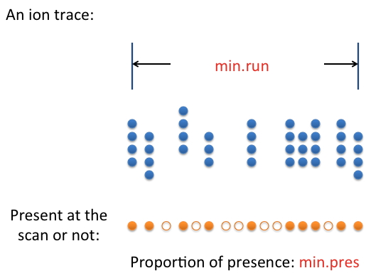
(1) min.run: the minimum footprint of a real feature in terms of retention time. It is closely related to the chromatography method used. How long should the retention time be for a real feature? Use that value or a value that's slightly smaller.

(2) min.pres: Sometimes the signal from a real feature isn't present 100% of the time along the feature's retention time. The parameter min.pres sets the threshold for an ion trace to be considered a feature. This parameter is best determined by examining the raw data.

min.run and min.pres explain, jpg

(3) mz.tol and align.mz.tol: these are m/z tolerance levels. For un-centroided data from FTMS machinery, these values are automaticly determined based on point distribution patterns in the data. However, for some lower-resolution data, especially when centroided, the automatic procedure may not yield the optimal result. Based on the machine's characteristics or examining the raw data - how far along m/z do two points need to be separated for them to be considered different? Use this value for mz.tol and align.mz.tol. An easy way is to use the machine's nominal resolution.

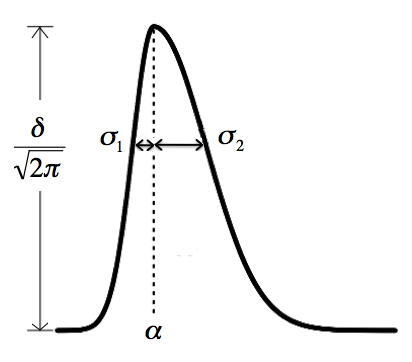
(4) sd.cut: this is a similar situation as min.run. It depends on how fast the elution of each peak is. This parameter (a vector of two numbers) sets the limits of the minimum and maximum standard deviation along rention time for an ion trace to be a real feature. Essentially four times the smaller value is the shortest retention time that is allowed, and four times the larger value is the longest retention time that's allowed. The picture below shows the bi-Gaussian model. It can be skewed to the other direction too. The sd.cut parameter sets the minimal and maximal value allow for either sigma.1 and sigma.2 in the picture.

explain bi gaussian, jpg

To aid parameter selection, we provide the function plot.2d() for the user to examine the detected features overlaid on the raw data. Set a small m/z and retention time range to zoom in to examine the pattern.

Critical parameters for determining features across multiple spectra in a project:

min.exp: If a feature is to be included in the final feature table, it must be present in at least this number of spectra.

Critical parameters for hybrid feature detection:

match.tol.ppm: The ppm tolerance to match identified features to known metabolites/features. Similar to mz.tol, this depends on the mass accuracy of your machine.

new.feature.min.count: The number of spectra a new feature must be present for it to be added to the database. We recommend setting this parameter in a stringent manner.

recover.min.count: The minimum time point count for a series of point in the EIC for it to be considered a true feature in supervised detection.

[Computation]

The computation time depends on the information contained in the spectra and the parameters. At the default setting, from one CDF file to its feature table, a laptop computer with a core 2 DUO CPU at 2.2 GHz takes about two minutes when the CDF file is about 30Mb. Retention time correction and feature alignment don't take too much time. Weaker signal recovery may take longer, as every spectrum is re-examined.

There are built-in mechanisms to speed up compuation.

(1) You can use multiple cores/machines to simultaneously perform steps 1 and 2 (from CDF file to per-spectrum feature table). The function cdf.to.ftr() has a pre-processing mode, in which it can work on only a subset of the CDF files, and save partially processed information in binary files. Later on, simply re-run the function cdf.to.ftr() or semi.sup() and it will look for the partially processed information in binary files and skip the first two steps if the files are present.

(2) Both and can utilize multiple cores on a machine. It is controlled by the n.nodes parameter in the wrapper functions. How many nodes you can use depends on two things: (1) the availability of cores in the machine, and (2) the size of RAM. A rule of thumb is to allow 2Gb RAM for each process.

[References]

apLCMS--adaptive processing of high-resolution LC/MS data. Yu T, Park Y, Johnson JM, Jones DP. Bioinformatics. 2009 Aug 1;25(15):1930-6.

Quantification and deconvolution of asymmetric LC-MS peaks using the bi-Gaussian mixture model and statistical model selection. Yu T, Peng H. BMC Bioinformatics. 2010 Nov 12;11:559.

A practical approach to detect unique metabolic patterns for personalized medicine. Johnson JM, Yu T, Strobel FH, Jones DP. Analyst. 2010 Nov;135(11):2864-70.

xMSanalyzer: automated pipeline for improved feature detection and downstream analysis of large-scale, non-targeted metabolomics data. Uppal K, Soltow QA, Strobel FH, Pittard WS, Gernert KM, Yu T, Jones DP. BMC Bioinformatics. 2013 Jan 16;14:15.

Hybrid feature detection and information accumulation using high-resolution LC-MS metabolomics data. Yu T, Park Y, Li S, Jones DP. J. Proteome Res. 2013 Mar 1; 12(3):1419-27.

Improving peak detection in high-resolution LC/MS metabolomics data using preexisting knowledge and machine learning approach. Yu T, Jones DP. Bioinformatics.2014 30(20): 2941-2948.